Logical query processing defines the conceptual interpretation of queries. A good understanding of this topic is key to writing correct and robust queries. During the last few months I provided an overview of the topic and described some of the major query clauses. In parts 2, 3, 4 and 5, I described the FROM clause and table operators.In part 6 I described the WHERE clause, and in part 7 I described the GROUP BY and HAVING clauses. In part 1 I also provided a sample database called TSQLV4 and two sample queries, which I referred to as simple sample query and complex sample query. This month I conclude the series by describing the last steps in logical query processing, which handle the SELECT and ORDER BY clauses, and the TOP and OFFSET-FETCH filters.
Complete logical query processing flow chart
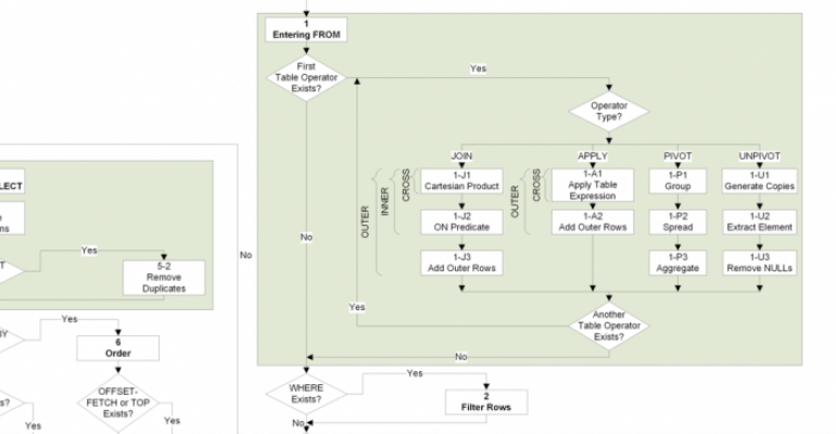
Figure 1 has the complete flowchart for logical query processing, including step 5, which handles the SELECT clause, step 6, which handles the ORDER BY clause, and step 7, which handles the TOP and OFFSET-FETCH filters.
Figure 1: Logical query processing flow chart - complete

Step 5, which evaluates the SELECT clause, operates on the result of step 4, which handles the HAVING filter. It can be broken into two substeps: step 5.1 evaluates the expressions in the SELECT list, and step 5.2 processes the DISTINCT clause, if present.
Step 6, which handles the ORDER BY clause, operates on the result of step 5 as its input. Without an ORDER BY clause in the outermost query, there’s no guarantee for the presentation ordering of the query result since the result is considered relational. With an ORDER BY clause in the outermost query, the result is considered nonrelational (a cursor), and presentation ordering is guaranteed.
Figure 1 also includes the handling of the TOP and OFFSET-FETCH filters, which can be considered as step 7. The TOP option filters the requested number, or percent, of rows based on the indicated ordering, if an ORDER BY clause is present. If an ORDER BY clause isn’t present, you should consider the order to be arbitrary. The OFFSET-FETCH filter requires an ORDER BY clause to be present. It skips the number of rows specified in the OFFSET clause and filters the number of rows specified in the FETCH clause, based on the defined ordering.
Let’s apply steps 5, 6 and 7 to our sample queries. Last month I described the output of step 4 in both sample queries. Recall that the output of step 4 is used as the input to step 5. Listing 1 has the complete simple sample query.
Listing 1: Simple sample query
USE TSQLV4; -- http://tsql.solidq.com/SampleDatabases/TSQLV4.zip

SELECT C.custid, COUNT( O.orderid ) AS numorders
FROM Sales.Customers AS C
  LEFT OUTER JOIN Sales.Orders AS O
    ON C.custid = O.custid
WHERE C.country = N'Spain'
GROUP BY C.custid
HAVING COUNT( O.orderid ) <= 3
ORDER BY numorders;
Following is the result of the HAVING clause, as described last month, and which is considered the input for step 5:
|---------|------------------|
| Groups  |       Rows       |
|---------|---------|--------|
|C.custid |C.custid |orderid |
|---------|---------|--------|
|     |8    |10326   |
|8    |8    |10801   |
|     |8    |10970   |
|---------|---------|--------|
|22       |22       |NULL    |
|---------|---------|--------|
Since the query is a grouped query, the rows in the result of step 4 are organized in groups. Step 5 evaluates the expressions from the SELECT list per group, resulting in two rows for the two groups, and step 6 presents those rows ordered by numorders. Here’s the final result of this query:
custid      numorders
----------- -----------
22      0
8       3
Since the ORDER BY clause appears in the outermost query, presentation ordering is guaranteed.
Listing 2 has the complete complex sample query.
Listing 2: Complex sample query
SELECT TOP (4) WITH TIES
  C.custid,
  A.custlocation,
  COUNT( DISTINCT O.orderid ) AS numorders,
  SUM( A.val ) AS totalval,
  SUM( A.val ) / SUM( SUM( A.val ) ) OVER() AS pct
FROM Sales.Customers AS C
  LEFT OUTER JOIN
  ( Sales.Orders AS O
      INNER JOIN Sales.OrderDetails AS OD
        ON O.orderid = OD.orderid
        AND O.orderdate >= '20160101' )
    ON C.custid = O.custid
  CROSS APPLY ( VALUES( CONCAT(C.country, N'.' + C.region, N'.' + C.city),
            OD.qty * OD.unitprice * (1 - OD.discount) )
      ) AS A(custlocation, val)
WHERE A.custlocation IN (N'Spain.Madrid', N'France.Paris', N'USA.WA.Seattle')
GROUP BY C.custid, A.custlocation
HAVING COUNT( DISTINCT O.orderid ) <= 3
ORDER BY numorders;
Here’s the state of the data before step 5 is applied:
|---------|----------------------------------------------------------------|
| Groups  |                Rows                |
|---------|---------|---------------|----------|-------------|-------------|
|C.custid |C.custid |A.custlocation |O.orderid |OD.productid |A.val    |
|---------|---------|---------------|----------|-------------|-------------|
|8    |8    |Spain.Madrid   |10970     |52       |224.0000000  |
|---------|---------|---------------|----------|-------------|-------------|
|22       |22       |Spain.Madrid   |NULL      |NULL     |NULL     |
|---------|---------|---------------|----------|-------------|-------------|
|57       |57       |France.Paris   |NULL      |NULL     |NULL     |
|---------|---------|---------------|----------|-------------|-------------|
|     |69       |Spain.Madrid   |10917     |30       |25.8900000   |
|     |69       |Spain.Madrid   |10917     |60       |340.0000000  |
|69       |69       |Spain.Madrid   |11013     |23       |90.0000000   |
|     |69       |Spain.Madrid   |11013     |42       |56.0000000   |
|     |69       |Spain.Madrid   |11013     |45       |190.0000000  |
|     |69       |Spain.Madrid   |11013     |68       |25.0000000   |
|---------|---------|---------------|----------|-------------|-------------|
|     |74       |France.Paris   |10907     |75       |108.5000000  |
|     |74       |France.Paris   |10964     |18       |375.0000000  |
|74       |74       |France.Paris   |10964     |38       |1317.5000000 |
|     |74       |France.Paris   |10964     |69       |360.0000000  |
|     |74       |France.Paris   |11043     |11       |210.0000000  |
|---------|---------|---------------|----------|-------------|-------------|
Also here the rows in the result of step 4 are organized in groups since the query is a grouped query. Currently there are five groups. Step 5 evaluates the expressions in the SELECT list, resulting in five rows. Notice the curious mix of grouping and windowing used in this query. The expression SUM( SUM( A.val ) ) OVER() computes the windowed grand total of the grouped total values. If you need a refresher for this capability, I explained it last month.
Step 6 defines ordering based on numorders (the distinct number of orders). The TOP option filters the first four rows based on numorders ordering. It also includes the WITH TIES option, which includes ties with the last row, if present. In our case, there are no ties with the last row, so the final query result has the following four rows:
custid  custlocation  numorders  totalval     pct
------- ------------- ---------- ------------ ---------
57      France.Paris  0      NULL     NULL
22      Spain.Madrid  0      NULL     NULL
8       Spain.Madrid  1      224.0000000  0.067431
69      Spain.Madrid  2      726.8900000  0.218818
Since the ORDER BY clause appears in the outermost query, presentation ordering is guaranteed.
The upcoming sections provide more detail on steps 5, 6 and 7.
Step 5: Process SELECT clause
As mentioned, step 5 handles the SELECT clause and can be broken into two substeps. Step 5.1 evaluates the expressions in the SELECT list, and substep 5.2 handles the DISTINCT clause.
Step 5.1: Evaluate expressions
Step 5.1 creates the heading of the relation that the query will eventually return. It evaluates the expressions in the SELECT list and assigns aliases to columns that are a result of a computation. If the query is a detailed query, this step generates one result row per input row. If the query is a grouped query, this step generates one result row per input group.
In the relational model the heading of a relation is a set of attributes. Since a set has no order and no duplicates, you identify an attribute by name and not by ordinal position. Plus, you can’t have duplicate attribute names. Depending on context, T-SQL—and the same applies to SQL—doesn’t always enforce such requirements. For instance, T-SQL allows a query to create an unnamed column that results from a computation, as the following example demonstrates:
SELECT C.custid, O.custid, O.orderid, YEAR(O.orderdate)
FROM Sales.Customers AS C
  LEFT OUTER JOIN Sales.Orders AS O
    ON C.custid = O.custid;
This query generates the following output:
custid      custid      orderid
----------- ----------- ----------- -----------
85      85      10248       2014
79      79      10249       2014
34      34      10250       2014
...
22      NULL    NULL    NULL
57      NULL    NULL    NULL
However, T-SQL does enforce both requirements as soon as you try to define a table expression such as a derived table, CTE, view or inline table-valued function, based on a query. For instance, the following attempt is invalid:
CREATE VIEW dbo.CustOrders
AS

SELECT C.custid, O.custid, O.orderid, YEAR(O.orderdate)
FROM Sales.Customers AS C
  LEFT OUTER JOIN Sales.Orders AS O
    ON C.custid = O.custid;
GO
The attempt to create this view fails.
To fix this, make sure you assign names to all columns, and that all column names are unique, like so:
CREATE VIEW dbo.CustOrders
AS

SELECT C.custid AS ccustid, O.custid AS ocustid, O.orderid, YEAR(O.orderdate) AS orderyear
FROM Sales.Customers AS C
  LEFT OUTER JOIN Sales.Orders AS O
    ON C.custid = O.custid;
GO
This time the view is created successfully.
Run the following for cleanup:
DROP VIEW dbo.CustOrders;
Also, as a reminder from discussions in previous months, all expressions that appear in the same logical query processing step are conceptually evaluated all-at-once as a set, and not in written order. This means that if you create an alias for a computation in the SELECT clause, that alias is not available to other computations in the same SELECT clause, rather only to expressions in subsequent logical query processing steps. For example, the following code is invalid:
SELECT orderid, YEAR(Orderdate) AS orderyear,
  DATEFROMPARTS(orderyear, 12, 31) AS endofyear
FROM Sales.Orders;
If you try running this query, you get the following error:
Msg 207, Level 16, State 1, Line 19
Invalid column name 'orderyear'.
To make an alias that is created by one computation available to another computation, you need to define the alias in a step that is earlier to the one that uses it. For example, you can create the alias using one CROSS APPLY operator, and use it in a second CROSS APPLY operator. You can then make available the results of the first and second operators to all subsequent steps, including WHERE, GROUP BY, HAVING and SELECT. Here’s the code that implements this technique:
SELECT orderid, orderyear, endofyear
FROM Sales.Orders
  CROSS APPLY ( VALUES( YEAR(Orderdate) ) ) AS A1(orderyear)
  CROSS APPLY ( VALUES( DATEFROMPARTS(orderyear, 12, 31) ) ) AS A2(endofyear);
Another important thing to remember about step 5.1 is that that’s the step where window functions are evaluated. That’s because a window function is supposed to operate on the underlying query result set (before removal of duplicates), and the underlying query result set is established only when you get to step 5. Prior to this step, the query result is still shaping. You’re not allowed to use window functions directly in earlier logical query processing steps. This means that if you need the use a window function in any step prior to step 5, you have to do this indirectly by using a table expression. For instance, suppose that you want to filter orders position at row numbers 21 through 30, based on orderid ordering. Since you cannot refer to the ROW_NUMBER window function directly in the WHERE clause, you need do so indirectly with a table expression, like so:
WITH C AS
(
  SELECT orderid, orderdate, custid, empid,
    ROW_NUMBER() OVER(ORDER BY orderid) AS rownum
  FROM Sales.Orders
)
SELECT orderid, orderdate, custid, empid
FROM C
WHERE rownum BETWEEN 21 AND 30;
The inner query computes row numbers in the SELECT clause and assigns the result column with the alias rownum. The outer query then refers to the rownum alias in the WHERE clause.
By the way, you cannot use the trick with the CROSS APPLY operator and the VALUES clause to assign aliases to computations based on window functions. That’s because the APPLY operator exposes to the right side only one row from the left, and window functions need to see the entire query result. So with window functions, you have to use the longer rout with the complete table expression such as with the last example.
Step 5.2: Process DISTINCT clause
If a DISTINCT clause is present in the SELECT clause, step 5.2 removes duplicates from the result of step 5.1. What’s interesting is that in relational theory a relation’s body is a set and hence can’t have duplicates. So, for instance, a query that projects only the country attribute of an Employee's relation is supposed to return only distinct countries where there are employees. T-SQL, as with SQL, deviates from the relational in that it allows duplicates in a table. Whereas the relational model is based in part on set theory, T-SQL is based on multiset theory. A multiset is similar to a set in the sense that it doesn’t have order, but different from a set in the sense that it allows duplicates. For one, you can create a table without a key, and therefore allow duplicate rows. For another, a query returning a subset of the columns could return duplicates. Consider the following query:
SELECT country FROM HR.Employees;
There are nine employees in the table, and therefore the query returns nine rows with duplicate countries:
country
---------------
USA
USA
USA
USA
UK
UK
UK
USA
UK
If you want to remove duplicates, you need to add an explicit DISTINCT clause, like so:
SELECT DISTINCT country FROM HR.Employees;
This query returns only two distinct countries:
country
---------------
UK
USA
Recall that that the DISTINCT clause is processed in step 5.2 and is applied after all expressions are evaluated in step 5.1. This means that if you have window functions, they’re evaluated before DISTINCT is applied. As an example, try to figure out how many rows the following query is supposed to return before running it.
SELECT DISTINCT country, ROW_NUMBER() OVER(ORDER BY country) AS rownum
FROM HR.Employees;
If you guessed two, you’re wrong. Prior to applying step 5.1, there are 9 rows in the input table for this step. This means that the ROW_NUMBER function generates 9 distinct row numbers in those 9 rows. Then the DISTINCT clause has no duplicates to remove, and you get the following output:
country     rownum
--------------- --------------------
UK          1
UK          2
UK          3
UK          4
USA         5
USA         6
USA         7
USA         8
USA         9
But what if you need to compute row numbers for distinct countries? One option is to write a query that returns only distinct countries, define a table expression based on that query, and then have the outer query compute row numbers for those distinct countries. Here’s the complete solution query:
WITH C AS
(
  SELECT DISTINCT country FROM HR.Employees
)
SELECT country, ROW_NUMBER() OVER(ORDER BY country) AS rownum
FROM C;
This query generates the following output:
country     rownum
--------------- --------------------
UK          1
USA         2
Another option is to use GROUP BY instead of DISTINCT. Remember that the GROUP BY clause is processed in step 3, well before step 5, which processes the SELECT clause. This means that any window functions are applied in step 5.1, after grouping. Here’s the complete solution query:
SELECT country, ROW_NUMBER() OVER(ORDER BY country) AS rownum
FROM HR.Employees
GROUP BY country;
You get only two rows in the result with the two distinct countries and their associated row numbers.
Step 6: Process ORDER BY clause
Without an ORDER BY clause in the query, the result is considered relational, and hence has no guaranteed order. If you need to guarantee presentation ordering in the result for purposes such as reporting, you must include an ORDER BY clause in the outermost query.
Since the ORDER BY clause is evaluated in step 6, after the SELECT clause, which is evaluated in step 5, you are allowed to refer to aliases that were created in the SELECT clause in the ORDER BY clause. This can be seen in both simple sample query and complex sample query. The SELECT clause computes the count of orders, aliasing it as numorders, then the ORDER BY clause refers to the numorders alias.
Normally, you are allowed to refer in the ORDER BY clause to expressions even if they don’t appear in the SELECT clause. In other words, you can order by things that you don’t necessarily want to return. The rule, though, is that you’re allowed to do this as long as the expression would have been valid if it were specified in the SELECT clause. The rules are stricter if you also use the DISTINCT clause. In such a case, the ORDER BY clause is limited only to expressions that appear in the SELECT clause. For example, the following query is invalid:
SELECT DISTINCT
  QUOTENAME(CONCAT(MONTH(orderdate), '/', YEAR(orderdate))) AS monthyear
FROM Sales.Orders
ORDER BY YEAR(orderdate), MONTH(orderdate);
The reasoning behind this restriction is that a single distinct value could represent multiple source rows, and then an expression in the ORDER BY clause could have different results for different source rows that are associated with the same target row. For example, think about a query that returns distinct countries and orders by the employee ID. There could be multiple different employee IDs associated with the same country. So T-SQL simply doesn’t support such queries. But what if you do have a one-to-one correlation between the results of the SELECT expressions and the ORDER BY expressions, as in the above query? The workaround is to apply distinctness without ordering in one query, define a table expression based on that query, and then handle the ordering in the outer query, like so:
WITH C AS
(
  SELECT DISTINCT MONTH(orderdate) AS ordermonth, YEAR(orderdate) AS orderyear
  FROM Sales.Orders
)
SELECT QUOTENAME(CONCAT(ordermonth, '/', orderyear)) AS monthyear
FROM C
ORDER BY orderyear, ordermonth;
This query generates the following output, shown here in abbreviated form:
monthyear
----------
[7/2014]
[8/2014]
...
[4/2016]
[5/2016]
ORDER BY, table expressions, TOP and OFFSET-FETCH
If you want to define a table expression such as a derived table, CTE, view or inline table valued function, the inner query is normally not allowed to have an ORDER BY clause. That’s because a table expression is supposed to represent a relation, and the result of a query with an ORDER BY clause is not relational. As an example, the following attempt to create a view is invalid:
CREATE VIEW Sales.MyView
AS

SELECT orderid, val
FROM Sales.Ordervalues
ORDER BY val DESC;
GO
If you run this code, it fails with the following error:
Msg 1033, Level 15, State 1, Procedure MyView, Line 6 [Batch Start Line 166]
The ORDER BY clause is invalid in views, inline functions, derived tables, subqueries, and common table expressions, unless TOP, OFFSET or FOR XML is also specified.
You're supposed to create the table expression based on the query without the ORDER BY clause and have the outer query against the table expression define presentation ordering. In other words, presentation ordering is supposed to be defined in the outermost query as the last thing before the result is returned to the caller.
If you read the error message carefully, you will notice that the restriction of no ORDER BY in the inner query is lifted in exceptional cases such as when you also specify the TOP or OFFSET-FETCH filters. These filters are applied to the result of step 5.2, and rely on the ORDER BY clause as if it were part of the specification of the filter. Theoretically, these filters could have been designed with their own ordering specification that is not confused with presentation ordering. But alas, that’s not the existing design. So when you use these filters in an inner query, you’re allowed to add an ORDER BY clause to support the filter. For example, the following view definition is valid:
CREATE VIEW Sales.MyView
AS

SELECT TOP (3) orderid, val
FROM Sales.Ordervalues
ORDER BY val DESC;
GO
But you need to remember the rule that I mentioned earlier with regards to presentation ordering—it’s only guaranteed if the outermost query has an ORDER BY clause. For example, consider the following query:
SELECT *
FROM Sales.MyView;
You are guaranteed to get the three orders with the highest values, but since the outer query doesn’t have an ORDER BY clause, you’re not guaranteed to get those rows presented in any specific order. Chances are that you will, since SQL Server uses an order based algorithm to handle TOP and OFFSET-FETCH to figure out which rows to filter. It’s not going to scramble the order of the rows just to present them sorted, because this will require more effort. Any order of the rows in the output is considered valid. So when I ran this query on my system, I got the following output, which seems to have the rows ordered by value, descending:
orderid     val
----------- ---------
10865       16387.50
10981       15810.00
11030       12615.05
However, there’s a big difference between what happens to be the order of the result due to optimization reasons versus what’s guaranteed to always be repeatable behavior. Physical processing and optimization choices can change.
A common mistake that people make is trying to create a “sorted view” by incorporating a TOP (100) PERCENT filter and an ORDER BY clause in the inner query, like so:
ALTER VIEW Sales.MyView
AS

SELECT TOP (100) PERCENT orderid, val
FROM Sales.Ordervalues
ORDER BY val DESC;
GO
The attempt is wrong to begin with because, as mentioned, a view is a relation and thus can’t have order. Moreover, when SQL Server optimizes a query against the view, it figures out that the combination of TOP (100) PERCENT and ORDER BY in the inner query is meaningless, and optimizes it out. For example, run the following query:
SELECT *
FROM Sales.MyView;
When I ran this query on my system, I got the following output, shown here in abbreviated form:
orderid     val
----------- --------
10248       440.00
10249       1863.40
10250       1552.60
10251       654.06
10252       3597.90
...
As you can see, the rows are not sorted by value, descending, and this isn’t a bug—it’s smart optimization. As mentioned, the only way to guarantee presentation order is with ORDER BY clause in outermost query.
If you combine the use of window functions and a TOP or OFFSET-FETCH filter in the same query, remember that window functions are applied in step 5.1 before the TOP and OFFSET-FETCH filters are applied—not the other way around. Consider the following example:
SELECT orderid, orderdate, custid, empid,
  ROW_NUMBER() OVER(ORDER BY orderdate, orderid) AS rownum,
  COUNT(*) OVER() AS totalrows
FROM Sales.Orders
ORDER BY orderdate, orderid
OFFSET 20 ROWS FETCH NEXT 10 ROWS ONLY;
Here the ROW_NUMBER function numbers the rows, and the COUNT(*) window function counts them before the OFFSET-FETCH filter is applied. Here’s the output of this query:
orderid  orderdate  custid  empid  rownum  totalrows
-------- ---------- ------- ------ ------- ----------
10268    2014-07-30 33      8      21      830
10269    2014-07-31 89      5      22      830
10270    2014-08-01 87      1      23      830
10271    2014-08-01 75      6      24      830
10272    2014-08-02 65      6      25      830
10273    2014-08-05 63      3      26      830
10274    2014-08-06 85      6      27      830
10275    2014-08-07 49      1      28      830
10276    2014-08-08 80      8      29      830
10277    2014-08-09 52      2      30      830
Observe that the result consists of the rows with row numbers 21 through 30 and not 1 through 10, and the totalrows column shows 830 and not 10. This may very well be the desired behavior, and then all is good. However, if you need to apply window functions to the result of a TOP or OFFSET-FETCH filter, use a table expression based on a query that applies the filter, and then apply the window functions in the outer query.
Conclusion
In this month’s article I focused on the SELECT and ORDER BY clauses, as well as considerations related to the TOP and OFFSET-FETCH filters. The series about logical query processing ended up having eight articles, and I’m sure I didn’t cover all that there is to say. It’s a big topic, and, to me, it's the most important topic to know about SQL. A good understanding of logical query processing results in writing correct and robust code.


