“There are known knowns. These are things we know that we know. There are known unknowns. That is to say, there are things that we know we don't know. But there are also unknown unknowns. There are things we don't know we don't know.” –Donald Rumsfeld (see YouTube video here.)
During query optimization, the optimizer applies cardinality estimates for operations like filters, joins, grouping, and so on to help in choosing from among the available processing strategies. When the user inputs are known and statistics are available, the optimizer can potentially make accurate cardinality estimates--and, consequently, optimal choices.
However, when statistics and user inputs are unavailable, the optimizer resorts to using a cardinality estimation technique called optimize for unknown. In such a case, calling the process estimating is probably a bit of an overstatement; it’s really more guessing than estimating. If you’re lucky, you’ll get estimates that are somewhat close to reality; if you aren’t lucky, you’ll get inaccurate estimates, which may lead to suboptimal choices.
In this article, I’ll provide the hard-coded guesses that the optimizer uses with the optimize for unknown technique so that at least you know what the optimizer guesses it doesn’t know. Good query tuning, in great part, starts with being able to explain cardinality estimations—especially ones that are inaccurate.
The famous Rumsfeld quote I opened the article with was his foot-in-mouth response to a reporter's question during a press conference held in 2002. The reporter then retorted: “Excuse me, but is this an unknown unknown?” To which Rumsfeld responded: “I’m not going to say which it is.”
In this article, I promise to say which it is--at least as far as optimizing for unknown is concerned--so that there won’t be any unknown unknowns left for you to worry about.
In my examples, I will query the Sales.SalesOrderDetail table in the AdventureWorks2014 sample database. If you want to run the examples from this article and don’t have this database installed, you can download it from codeplex here. You will also want to make sure that the database is set to compatibility mode 120 to ensure that SQL Server will use the new cardinality estimator (2014) by default. You can do this by running the following code:
-- Make sure db compatability is >= 120 to use new CE by default
USE AdventureWorks2014; -- https://msftdbprodsamples.codeplex.com/releases/view/125550
GO

IF ( SELECT compatibility_level
     FROM sys.databases
     WHERE name = N'AdventureWorks2014' ) < 120
  ALTER DATABASE AdventureWorks2014
    SET COMPATIBILITY_LEVEL = 120; -- use 130 on 2016
I’ll break down the optimize for unknown estimates by the following groups of operators:
- >, >=, <, <=
- BETWEEN and LIKE
- =
In the first section where I cover the first group of operators, I’ll also demonstrate the different scenarios where the optimizer uses the optimize-for-unknown technique. In subsequent sections I’ll just use one or a couple of the scenarios to demonstrate the estimates.
Optimize for unknown estimates for the operators: >, >=, <, <=
The optimize-for-unknown estimate for the group of operators >, >=, < and <= is 30 percent of the input’s cardinality. That’s the case with both the new cardinality estimator (2014) and the legacy one (7.0).
For example, suppose you query the Sales.SalesOrderDetail table in the AdventureWorks2014 database, and you use a filter such as WHERE OrderQty >=
Since this is the first section in which I’m demonstrating the optimize for unknown technique, let me start by listing the different cases where this technique is used along with runnable examples.
The optimize for unknown technique is used:
1. When using local variables.
Unlike parameter values, which are sniffable, variable values normally are not sniffable. (I’ll describe an exception shortly.) The reason is simple: The initial optimization unit is the entire batch—not just the query statement. Variables are declared and assigned with values as part of the batch that gets optimized. The point when the query gets optimized is before any variable assignment took place, and hence variable values can’t be sniffed. The result is that the optimizer has to resort to using the optimize for unknown technique.
To compare the optimize-for-unknown technique with the natural optimize for known technique, consider the following query, which has a filter predicate with the >= operator and a known constant as the input:
SELECT ProductID, COUNT(*) AS NumOrders

FROM Sales.SalesOrderDetail

WHERE OrderQty >= 40

GROUP BY ProductID;
The execution plan that I got for this query is shown in Figure 1.
Figure 1: Query plan for query with a constant

Here the classic tool that the optimizer used to make the cardinality estimation for the filter is a histogram. If one didn’t exist on the OrderQty column before you ran this query and you didn’t disable automatic creation of statistics in the database, SQL Server created one when you ran the query. You can use the query in Listing 1 to get the automatically created statistics name.
Listing 1: Identify automatically created statistics on OrderQty column
SELECT S.name AS stats_name

FROM sys.stats AS S

  INNER JOIN sys.stats_columns AS SC

ON S.object_id = SC.object_id

   AND S.stats_id = SC.stats_id

  INNER JOIN sys.columns AS C

ON SC.object_id = C.object_id

   AND SC.column_id = C.column_id

WHERE S.object_id = OBJECT_ID(N'Sales.SalesOrderDetail')

  AND auto_created = 1

  AND C.name = N'OrderQty';
When I ran this code after running the previous query I got the statistics name _WA_Sys_00000004_44CA3770. Make a note of the one that you got. Then use the following code to see the histogram, after replacing the statistics name with the one that you got:
DBCC SHOW_STATISTICS (N'Sales.SalesOrderDetail', N'_WA_Sys_00000004_44CA3770')

  WITH HISTOGRAM;
The last few steps in the histogram that I got are shown in Table 1.
Table 1: Last few histogram steps
RANGE_HI_KEY RANGE_ROWS    EQ_ROWS       DISTINCT_RANGE_ROWS  AVG_RANGE_ROWS
------------ ------------- ------------- -------------------- --------------
...
38       0         1         0            1
39       0         1         0            1
40       0         2.006392      0            1
41       0         1         0            1
44       0         1         0            1
You can very clearly see how the cardinality estimate shown in Figure 1 was based on the last three steps of the histogram. The estimate is pretty accurate: 4.00639 versus an actual of 4.
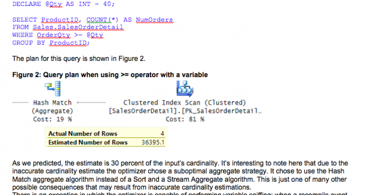
In contrast to the above example, the following query uses a local variable, forcing the optimizer to use the optimize for unknown technique:
DECLARE @Qty AS INT = 40;


SELECT ProductID, COUNT(*) AS NumOrders

FROM Sales.SalesOrderDetail

WHERE OrderQty >= @Qty

GROUP BY ProductID;
The plan for this query is shown in Figure 2.
Figure 2: Query plan when using >= operator with a variable

As we predicted, the estimate is 30 percent of the input’s cardinality. It’s interesting to note here that, due to the inaccurate cardinality estimate, the optimizer chose a suboptimal aggregate strategy. It chose to use the Hash Match aggregate algorithm instead of a Sort and a Stream Aggregate algorithm. This is just one of many other possible consequences that may result from inaccurate cardinality estimations.
There is an exception in which the optimizer is capable of performing variable sniffing: when a recompile event happens at the statement level. That’s because, by definition, a statement-level recompile happens after any variable assignments already took place. Automatic recompiles always happen at the statement level. This has been the case all the way since SQL Server 2005 and until the date of this writing (I’m testing the code on SQL Server 2016). To get a manual statement-level recompile, you need to add the RECOMPILE query hint using the OPTION clause, like so:
DECLARE @Qty AS INT = 40;


SELECT ProductID, COUNT(*) AS NumOrders

FROM Sales.SalesOrderDetail

WHERE OrderQty >= @Qty

GROUP BY ProductID

OPTION (RECOMPILE);
This query generates the same plan as the one shown earlier in Figure 1, where the estimate is accurate.
Note that if you specify the procedure level WITH RECOMPILE option, it won’t enable variable sniffing—only the query hint OPTION(RECOMPILE) does.
The optimize for unknown technique is also used:
2. When using parameters but disabling the automatic parameter sniffing by specifying OPTIMIZE FOR UNKNOWN or OPTIMIZE FOR (@parameter UNKNOWN) or with the trace flag 4136.
Normally parameter values are sniffable since you assign them with values in the execution of the procedure or function before the batch is passed to the optimizer for optimization. However, you can force the optimize for unknown technique with a couple of query hints. If you want to disable parameter sniffing for all inputs, use the hint OPTIMIZE FOR UNKNOWN. If you want to disable sniffing of a specific parameter, use the hint OPTIMIZE FOR (@parameter UNKNOWN). You can also use trace flag 4136 to disable parameter sniffing at different granularities: query, session or globally. Note that when using natively compiled stored procedure, the optimize-for-unknown behavior is the default by design.
As an example, the following code create a stored procedure and disables parameter sniffing in the query using the OPTIMIZE FOR UNKNOWN hint:
IF OBJECT_ID(N'dbo.Proc1', N'P') IS NOT NULL DROP PROC dbo.Proc1;

GO

CREATE PROC dbo.Proc1

  @Qty AS INT

AS


SELECT ProductID, COUNT(*) AS NumOrders

FROM Sales.SalesOrderDetail

WHERE OrderQty >= @Qty

GROUP BY ProductID

OPTION (OPTIMIZE FOR UNKNOWN);

GO
Use the following code to test the stored procedure:
EXEC dbo.Proc1 @Qty = 40;
I got the same query plan like the one shown earlier in Figure 2, showing a 30 percent cardinality estimate.
Another scenario where the optimize for unknown technique is used is:
3. When statistics are unavailable.
Consider a case where there’s no histogram available on the filtered column, and you prevent SQL Server from creating one by disabling automatic creation of statistics at the database level and by not creating an index on the column. Use the following code to arrange such an environment for our demo, after replacing the statistics name with the one that you got by running the query I provided earlier in Listing 1:
ALTER DATABASE AdventureWorks2014 SET AUTO_CREATE_STATISTICS OFF;

GO

DROP STATISTICS Sales.SalesOrderDetail._WA_Sys_00000004_44CA3770;
Next, use the following code which uses a constant in the filter:
SELECT ProductID, COUNT(*) AS NumOrders

FROM Sales.SalesOrderDetail

WHERE OrderQty >= 40

GROUP BY ProductID;
When you ran this query earlier, you got the plan shown in Figure 1 with an accurate cardinality estimate. But this time since the optimizer has no histogram to rely on, it uses the optimize for unknown technique and creates the plan shown earlier in Figure 2 with the 30 percent estimate.
Run the following code to re-enable auto creation of statistics in the database:
ALTER DATABASE AdventureWorks2014 SET AUTO_CREATE_STATISTICS ON;
You can rerun the query and see that you get the plan in Figure 1.
Optimize for unknown estimates for the BETWEEN and LIKE operators.
When using the BETWEEN predicate the hard-coded guess depends on the scenario and the cardinality estimator (CE) that is being used. The legacy CE uses a 9 percent estimate in all cases. The following query demonstrates this. (Query trace flag 9481 is used to force the legacy CE.):
DECLARE @FromQty AS INT = 40, @ToQty AS INT = 41;


SELECT ProductID, COUNT(*) AS NumOrders

FROM Sales.SalesOrderDetail

WHERE OrderQty BETWEEN @FromQty AND @ToQty

GROUP BY ProductID

OPTION(QUERYTRACEON 9481);
The plan for this query is shown in Figure 3. The estimate is 0.09 * 121317 = 10918.5.
Figure 3: Plan showing a 9 percent estimate

The new CE uses different estimates when using constants and a histogram is unavailable and when using variables or parameters with sniffing disabled. For the former it uses an estimate of 9 percent; for the latter it uses an estimate of 16.4317 percent.
Here’s an example demonstrating the use of constants. (Make sure you drop any existing statistics on the column and disable automatic creation of statistics as shown earlier before you run the test and re-enable it after the test.):
DECLARE @FromQty AS INT = 40, @ToQty AS INT = 41;


SELECT ProductID, COUNT(*) AS NumOrders

FROM Sales.SalesOrderDetail

WHERE OrderQty BETWEEN @FromQty AND @ToQty

GROUP BY ProductID

OPTION(QUERYTRACEON 9481);
I got the same plan as the one shown earlier in Figure 3 with the estimate of 9 percent.
Here’s an example demonstrating the use of variables (same behavior when using parameters with sniffing disabled):
DECLARE @FromQty AS INT = 40, @ToQty AS INT = 41;


SELECT ProductID, COUNT(*) AS NumOrders

FROM Sales.SalesOrderDetail

WHERE OrderQty BETWEEN @FromQty AND @ToQty

GROUP BY ProductID;
I got the plan shown in Figure 4, showing a 16.4317 percent estimate.
Figure 4: Plan showing a 16.4317 percent estimate

When using the LIKE predicate in all optimize for unknown scenarios both the legacy and new CEs use a 9 percent estimate. Here’s an example using local variables:
DECLARE @Carrier AS NVARCHAR(50) = N'4911-403C-%';


SELECT ProductID, COUNT(*) AS NumOrders

FROM Sales.SalesOrderDetail

WHERE CarrierTrackingNumber LIKE @Carrier

GROUP BY ProductID;
You will see the same 9 percent estimate as the one shown earlier in Figure 3, although in this case the actual number of rows is 12 and earlier it was 3.
Optimize for unknown estimates for the = operator
When using the = operator there are three main cases:
- Unique column
- Non-unique column and density available
- Non-unique column and density unavailable
When the filtered column is unique (has a unique index, PRIMARY KEY or UNIQUE constraint defined on it), the optimizer knows there can’t be more than one match, so it simply estimates 1. Here’s a query demonstrating this case:
DECLARE @rowguid AS UNIQUEIDENTIFIER = 'B207C96D-D9E6-402B-8470-2CC176C42283';


SELECT *

FROM Sales.SalesOrderDetail

WHERE rowguid = @rowguid;
Figure 5 has the plan for this query showing an estimate of 1.
Figure 5: Estimate of 1 for = operator with a unique column

When the column is non-unique and density (average percent per distinct value) information is available to the optimizer, the estimation will be based on the density. If you didn’t turn off automatic creation of statistics or have an index created on the column, this information will be available to the optimizer. To demonstrate this, first make sure automatic creation of statistics is on by running the following code:
ALTER DATABASE AdventureWorks2014 SET AUTO_CREATE_STATISTICS ON;
Then run the following query:
DECLARE @Qty AS INT = 1;


SELECT ProductID, COUNT(*) AS NumOrders

FROM Sales.SalesOrderDetail

WHERE OrderQty = @Qty

GROUP BY ProductID;
Figure 6: Plan showing estimate based on density

Remember that density is the average percent per distinct value in the column. It’s calculated as 1 /
DBCC SHOW_STATISTICS (N'Sales.SalesOrderDetail', N'_WA_Sys_00000004_44CA3770')
  WITH DENSITY_VECTOR;
I got the following output:
All density   Average Length Columns
------------- -------------- ----------
0.02439024    2          OrderQty
You realize that this method based on density is generally good for you when indeed the inputs you query most often have a cardinality that is close to the average cardinality. Clearly that’s not our case in the last example. The quantity 1 appears more often than the average, so the actual number is greater than the estimate.
When using a non-unique column and density isn’t available, the legacy CE and new CE use slightly different methods. The legacy CE uses an estimate of C^0.75 (an exponent of three quarters), where C is the input’s cardinality, whereas the new CE use an estimate of C^0.5 (the square root).
To demonstrate this first remove any statistics on the OrderQty column and turn off automatic creation of statistics as shown before:
ALTER DATABASE AdventureWorks2014 SET AUTO_CREATE_STATISTICS OFF;

GO

DROP STATISTICS Sales.SalesOrderDetail._WA_Sys_00000004_44CA3770;
Use the following code to test the legacy CE method:
DECLARE @Qty AS INT = 1;


SELECT ProductID, COUNT(*) AS NumOrders

FROM Sales.SalesOrderDetail

WHERE OrderQty = @Qty

GROUP BY ProductID

OPTION(QUERYTRACEON 9481);
The plan for this query is shown in Figure 7.
Figure 7: Plan showing legacy CE estimate of C^3/4

The estimate of 6500.42 is the result of 121317^3/4.
Use the following code to test the new CE method:
DECLARE @Qty AS INT = 1;


SELECT ProductID, COUNT(*) AS NumOrders

FROM Sales.SalesOrderDetail

WHERE OrderQty = @Qty

GROUP BY ProductID;
The plan for this query is shown in Figure 8.
Figure 8: Plan showing new CE estimate of C^0.5

The estimate of 348.306 is the result of 121317^0.5.
When you’re done testing, make sure you re-enable automatic creation of statistics by running the following code:
ALTER DATABASE AdventureWorks2014 SET AUTO_CREATE_STATISTICS ON;
Summary
The optimize-for-unknown technique is used by the SQL Server optimizer to make cardinality estimates for unknown inputs or lack of statistics. Sometimes the optimizer has no choice but to use this method simply because it’s missing information, and sometimes you want to force it when the optimize-for-known technique is bad for you. This article had lots of detail. For reference purposes, the following two items summarize what the article covered.
The optimize for unknown technique is used in any of the following scenarios:
1. Using variables (unless statement-level RECOMPILE used)
2. Using parameters with: OPTIMIZE FOR UNKNOWN or OPTIMIZE FOR (@parameter UNKNOWN) hint or TF 4136 (always the case with natively compiled stored procedures)
3. Statistics are unavailable
Table 2 has the summary of the optimize-for-unknown estimates used for the different groups of operators.
Table 2: Optimize for unknown estimates for operators


