![]() In a simple and easy-to-understand format, this article provides the necessary steps to creating a Power Pivot Data Model in Microsoft Excel 2013, as well as instruction on how to generate a complex report in Excel using a Power Pivot table.
In a simple and easy-to-understand format, this article provides the necessary steps to creating a Power Pivot Data Model in Microsoft Excel 2013, as well as instruction on how to generate a complex report in Excel using a Power Pivot table.
Related: Understanding Power Pivot and Power View in Microsoft Excel 2013
If you are using Excel 2013, Power Pivot is installed by default. If not, you can install it by going to:
Files → Options → Add-ins (This is a tab on the left panel of the screen.)
In the Manage dropdown list, select COM Add-Ins and press Go.

After pressing the Go button, a new screen will open in front of you. Select Microsoft Office Power Pivot for Excel 2013. This will add a new ribbon tab in your Excel ribbon menu as Power Pivot.

Excel 2010
If you are using Excel 2010, you will have to download the Power Pivot setup. Make sure to check the prerequisites and system requirements for Power Pivot for Excel 2010 before installation.
Sample Database
Use the provided sample database script available at the top of the page via the "Download the Code" icon. All you have to do is copy the script and paste it into the new query window of your SQL Server Management Studio (SSMS) and select Execute.
Overview
In this exercise, you will be developing a Power Pivot model by importing SQL Server data into Excel. We will create hierarchies, calculated columns, Key Performance Indicators (KPIs), and add related columns on the basis of DAX language.
The Excel document will look like this:

Step 1: Load Data
In this step, you'll load data from SQL Server database (DWtest) into Excel 2013 file. To do this, perform the following steps:
1. Create a new Excel 2013 Workbook.
2. Go to the Power Pivot ribbon tab and select the Manage menu item. This will open a new Power Pivot for Excel window. In this screen, we will design our data model.
3. On the Home ribbon tab, select From Database and then select From SQL Server. This will start the table import wizard. On the first screen, you'll specify the connection parameters (Server Name, Log On to Server and Database Name) with your SQL Server Instance on which you have deployed the Sample Database. I have selected '.\sql2012' as my Server. (The peridod "." indicates that the server is my localhost. sql2012 is my instance name where my database DWTest is deployed.)
I have chosen the Windows Authentication as my connection authentication. Your first screen looks like this:

4. By hitting the Next button, you'll be asked for how to import your tables. Leave the default option selected: Select from a list of tables and views to choose the data to import. Select Next.

5. On the next screen, you'll be provided the list of tables in the database that you selected in the first screen of the wizard.
6. Select all tables except sysdiagram and FactTrainingBooking.
7. You can specify friendly names for each table by typing in the Friendly name column in front of each table name. You can also filter the columns that you need to import to your data model by selecting table name and then select Preview and Filter. You can uncheck the columns that you don't need to import in your data model. You can also hide columns and tables in the data model.


The Applied Filters hyperlink is there because you have unchecked the CityKeyID column of this table. Therefore, it will not be imported into the model.
8. Select Finish. This will process the selected tables. No error should be generated in this step. By clicking the Details hyperlink in the last row of the Details grid, you'l notice the relationships inherited by the wizard from the OLTP database design within the selected tables.

9. Select Close to close the window. This will populate your Power Pivot for Excel screen.
Step 2: Explore the Imported Model
From the screen, you'll notice that each table is presented with the tab at the bottom. You can rename the tab by right-clicking the respective tab and select Rename.
Also, you can hide columns by right-clicking the respective column header and select Hide from Client Tool'. You can also hide the entire table in this way.
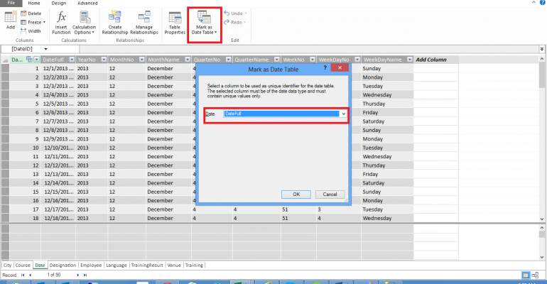
Step 3: Marking the Date Table
In this step, you'll inform the model about your date table. Follow these steps;
1. Select Date table.
2. Select Mark as Date Table and then click Mark as Date Table. This action will open a screen.

The selected column in the opened screen is the DateFull column containing full date. Click OK.
Step 4: Creating Related Columns
Select the Employee table and perform the following steps:
1. Select Design ribbon item and select Add in Columns group.
2. This will take the cursor in the formula bar.
3. Add the following code in the formula bar: =RELATED(Designation[DesignationDesc])
This will add the designation descriptions in the Employees table from the Designation table on the basis of the relationships defined.
4. You can add City and Language in the same way.
Step 5: Adding Hierarchies
To add hierarchies:
1. Switch to the diagram view by clicking  button at the right bottom of the screen.
2. This will open the model in the diagram view. Here you can perform different tasks by right-clicking the tables and columns. Maximize the Date table by clicking Maximize button.
3. Add Hierarchy in Date table as Calendar by right-clicking YearNo column and select Create Hierarchy. This will add a new hierarchy at the bottom. You can rename it as Calendar by right-clicking, and then select Rename.
4. Right-click on QuarterName and select Add to Hierarchy and then Calendar.
5. Do the same with MonthName, as in step 4.
6. Hide the rest of the columns on the date table other than the newly created hierarchy as you don't need them. Click the first column. Press shift key and while holding the shift key, click the last column, right above the hierarchy. Right click and the select Hide from Client Tools.
7. Click the Restore button at the top of the Date table. This will return the view of the table back to normal.
8. Hide All the ID columns from all tables to get a better user-friendly look of the model in Excel.
Step 6: Adding Measures
Select the Training table and do the following:
1. Right click the table Header and select Go to. This will return you to the Grid view from the Diagram view.
2. Select cell at the bottom of the TrainingID column. In Home ribbon tab, go to Calculations group and click the AutoSum dropdown. Select Count from the dropdown list. This will add Count Measure on TrainingID Column
3. Select all columns of the Training table, except Score, and hide them from client tools by right clicking them.
4. Select the empty cell at the bottom of the score column. Add Average measure as illustrated in step 2.
5. Go to the Home ribbon tab. In the Formatting section, change the Format of the measure to Decimal Number.
6. You can edit the text of the measure by editing the first portion of the formula in the formula bar. For the just added Average of Score measure, go the formula bar and edit the text before ':=' as Average. This will change the caption of the measure.
Step 7: Adding KPI
1. Right click Average measure. Select Create KPI. This will open a new window.

2. Select Absolute Value. Type 100 as the value.
3. Type 60 in the first box of the thresholds and type 80 in the second box.
4. Click OK.
Step 8: Draw the Model in Excel for Power Pivot Report
1. Go to Home ribbon tab and select Pivot Table and then select Pivot Table again.

2. This will prompt a screen. Select Existing worksheet as in the screen below.

Click OK. This will draw a Pivot Table on the basis of our designed model in the Excel file. Here you can play around with the pivot table. You can still make changes in your Power Pivot model. These changes will reflect in the Excel file automatically.
3. Select Calendar hierarchy in Date table and add it in the Filters. Select Filter from the Excel cell and Select 2013 instead of All.
4. Select CourseName field from Course table and add it in ROWS area. This will add the list of courses in the in the pivot table.
5. Select TrainingresultDesc from TrainingResult Table.
6. Select Score field from Training Table. This will add a column Sum of Score in the Pivot table.
7. Select Value and Status field from Average KPI in Training table. This will lead you to the required report.
Summary
In this exercise, you created a Power Pivot Data Model on SQL Server OLTP database data. You added related columns, measures, hierarchies, and KPI in the model and generated a quick pivot table-based report in Excel 2013. This practice is called Self-Service BI. By practicing, you'll learn that the steps are simple and the interface is user-friendly.
You can design more complex Power Pivot Models in Excel 2013, but there are some drawbacks. The data is not managed. You have to share the Excel file to a SharePoint Server to share with your peers, or you might face data and connectivity problems. There are also data integrity issues. That's where Tabular Model comes into play. Tabular Model is a part of Corporate-Business Intelligence (BI)—it's centrally deployed and you can manage permissions to give access to the data in the model.
**************************************************************************************
Atif-ullah Sheikh is a Database Architect and Consultant for the Microsoft Practice at En Pointe Technologies, an IT solutions provider based in Gardena, California. Sheikh's areas of expertise include SQL Server Database Design and Development, Business Intelligence, Analysis Services, Reporting Services, Integration Services, SQL Database, Big Data, MS Excel, Power Pivot, Power Query, and Power View.
Email: [email protected]
***************************************************************************************


